Estimating Load Capacity and Test Throughput of Environmental Test Chambers for PV Modules - Part 1

1. Background and Problem Definition

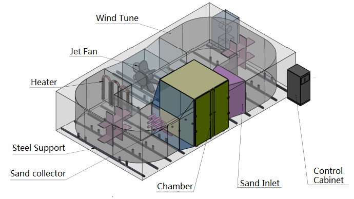
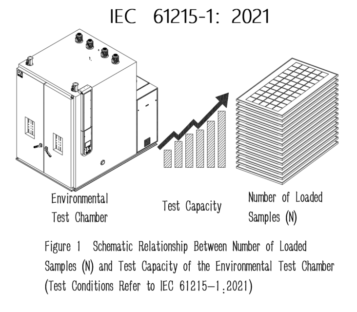
In environmental testing of photovoltaic (PV) modules, the number of modules that can be loaded into a test chamber in a single batch directly affects not only the batch capacity and overall test cycle, but also temperature uniformity and the load on the refrigeration system.

If the loading quantity is too low, equipment utilization and test throughput remain inefficient. If the loading quantity is too high, the temperature ramp rate may fail to meet the required specification, and temperature uniformity may deteriorate significantly.

In current engineering practice, loading decisions are still often based on empirical recommendations, such as a “suggested number of modules” for a given chamber type. However, these recommendations are frequently detached from key boundary conditions, including chamber dimensions, airflow configuration, temperature ramp rate, and refrigeration system capacity. Once any of these parameters change, empirical values become difficult to reuse and are unsuitable for comparison across different projects.

Against this background, this article attempts to establish a systematic framework around the chain of loading quantity – temperature uniformity – cooling capacity – test efficiency, focusing on the following aspects:

• Under a given temperature ramp rate and uniformity requirement, integrating the thermal capacity of air, fixtures, PV modules, and chamber heat transfer into a unified heat balance framework;

• Accounting for airflow rate and airflow organization to derive the effective usable cooling capacity of the refrigeration system;

• Based on this framework, determining the maximum safe loading quantity $n_{max}$, and further estimating the theoretical test throughput and test cycle.

By combining heat balance and air distribution into a simplified engineering model, this approach aims to provide a unified calculation method for evaluating chamber loading capacity across different projects. It supports early-stage estimation during design and equipment selection, and also serves as a quantitative basis when explaining test efficiency and scheduling to end users.

2. Definition of Ramp Rate and Scope of This Article

Before discussing “how many modules can be loaded at most,” the definition of temperature ramp rate must be clarified.

For the same chamber, the allowable loading quantity under 3.3 ℃/min and 1.67 ℃/min is fundamentally different. A single loading conclusion cannot be applied across different ramp rates.

2.1 Two Commonly Used Ramp Rates

In engineering practice, two reference ramp rates are commonly used:

• 3.3 ℃/min: Capability condition, used to evaluate performance under higher ramp rates, and convenient for estimating production rhythm and test throughput;

• 1.67 ℃/min (approximately 100 ℃/h): Standard condition, corresponding to IEC and other environmental test standards, where many test clauses are defined at this rate.

For clarity, all examples in this article are calculated at 3.3 ℃/min. For standard compliance verification, the ramp rate can simply be replaced with 1.67 ℃/min, while all other calculation steps remain unchanged.

In the following formulas:

• Temperature is expressed in ℃;

• Ramp rate in ℃/min;

• Heat capacity in kJ/℃;

• Power in kW.

Units are not repeatedly stated unless otherwise specified.

The upper limit of loading capacity is essentially the intersection of demand-side heat load and supply-side cooling capacity under the most unfavorable operating condition.

3. Core Concept: Heat Balance and Air Distribution

3.1 Demand Side: Unified Heat Balance

For environmental tests discussed in this article (such as thermal cycling, damp heat, and humidity freeze), PV modules typically carry only small measurement or monitoring currents. The corresponding electrical power is negligible compared to the kW-level thermal load associated with temperature ramping and heat transfer, and can be ignored in engineering calculations.

Therefore, instead of separately considering “self-heating of modules,” all contributions are integrated into a unified framework, including:

• Equivalent heat capacity of air $C_{air}$;

• Heat capacity of fixtures and inner chamber structures $C_{fixtures}$;

• Equivalent heat capacity of PV modules $C_{panel}$;

• Chamber heat transfer term $UA \cdot \Delta T$;

• Minor internal heat sources and leakage loads $Q_{misc}$.

During the temperature ramp phase, the demand-side thermal load can be expressed as:

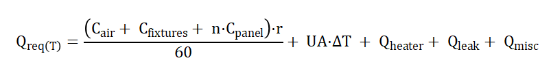
Where:

• $n$: number of loaded modules;

• $r$: temperature ramp rate (℃/min);

• $C_{air}, C_{fixtures}, C_{panel}$: equivalent heat capacities of air, fixtures/inner chamber, and a single PV module (kJ/℃);

• $UA \cdot \Delta T$: heat transfer load through chamber walls;

• $Q_{heater}$: additional load from door heaters, observation windows, etc. (treated as negative cooling capacity);

• $Q_{leak}$: heat leakage due to door opening or imperfect sealing;

• $Q_{misc}$: other internal heat sources such as lamps or instrumentation.

3.2 Supply Side: Refrigeration Capacity and Airflow Utilization

The supply-side cooling capacity can be expressed as:

Where:

• $Q_r(actual)$ is the nominal compressor cooling capacity derated under actual evaporating temperature, condensing temperature, superheat/subcooling conditions, and airflow or water flow conditions;

• $\eta(V)$ is the utilization efficiency dependent on airflow rate and airflow rectification, reflecting factors such as evaporator surface utilization, frosting or condensation effects, return-air organization, and short-circuit airflow.

In intuitive terms, even with the same refrigeration system, insufficient airflow or severe airflow short-circuiting can significantly reduce the effective cooling capacity delivered to the working zone.

4. Why “Airflow” and “Spacing” Often Become the Bottleneck

In PV module environmental testing, many cases of “poor uniformity after increasing loading” are not caused solely by insufficient cooling capacity. More often, they result from the combined effects of inadequate airflow organization and excessively tight module spacing.

From a heat transfer perspective, PV modules dissipate heat mainly through convection, which can be simplified as:

Where:

• $\alpha$ is the overall convective heat transfer coefficient, determined by airflow velocity and surface conditions;

• $A_{eff}$ is the effective surface area exposed to airflow;

• $\Delta T$ is the temperature difference between the module surface and the air.

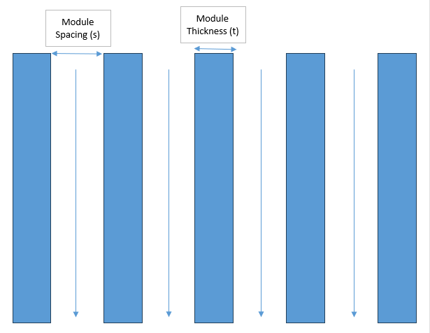
For bifacial heat exchange of PV modules, the effective area can be expressed as:

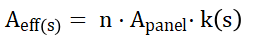
Where:

• $A_{panel}$ is the single-side area of one module;

• $k(s)$ is a spacing correction factor dependent on module spacing $s$, reflecting the degree to which the rear side is effectively exposed to airflow.

When spacing is very small and the rear side is nearly blocked, airflow mainly sweeps over the front surface, and $k(s)$ approaches 1. As spacing increases and airflow penetrates between modules, the rear side increasingly participates in heat exchange, and $k(s)$ approaches 2.

Based on existing project experience, for modules with thickness $t \approx 35$ mm, maintaining a spacing of $s \ge 50\text{–}60$ mm along the main airflow direction allows rear-side airflow penetration in most chambers, yielding $k(s) \approx 1.6\text{–}1.8$. If spacing is compressed too much, even with seemingly sufficient total airflow, the middle modules often remain in low-velocity zones, reducing $A_{eff}$ and causing higher or slower temperature response.

Therefore, when investigating non-uniformity at high loading, the recommended sequence is:

1. Check airflow paths: supply and return airflow, and whether short-circuiting exists;

2. Check spacing: whether modules are overly compressed along the main airflow direction;

3. Only after these conditions are satisfied should cooling capacity and loading quantity be further discussed.

Airflow determines whether heat can be removed at all; spacing determines whether both sides of the modules are truly exposed to airflow.

5. Calculation Procedure: Four Steps to Determine $n_{max}$

Without predefining the loading quantity, the recommended upper limit $n_{max}$ can be obtained through the following four steps.

Step 1: Determine peak demand.
Using the heat balance equation, calculate $Q_{req}(T)$ at key temperatures such as +60 ℃, +25 ℃, −20 ℃, and −40 ℃, or determine the envelope over the entire temperature range to identify the most unfavorable condition.

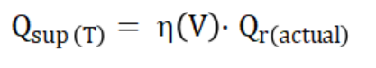
Step 2: Determine available cooling capacity.
Derate the nominal compressor capacity to actual operating conditions, then multiply by airflow utilization efficiency to obtain:

Q_sup(T) = η(V)·Q_r(actual)。

Step 3: Solve for loading limit.
Rearranging the heat balance equation for the ramp phase yields the recommended loading upper limit:

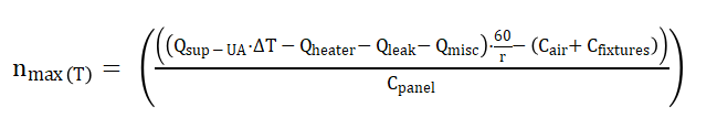
Step 4: Verify airflow and uniformity.
After obtaining $n_{max}$, verify airflow rate, velocity, and measured temperature uniformity. Adjust spacing, airflow paths, or airflow rate if necessary.

Based on $n_{max}$ and actual scheduling parameters, theoretical throughput can then be estimated by combining batch size, test duration per batch, changeover time, and operating shifts.

To Be Continue......